Examples
The examples below demonstrate how to use the spectra_processor class to generate the spectra continuum flux and identify specific abosrption features.
The spectra for one SDSS QSO at a redshift of z=1.8449 can be downloaded here.
This sightline constains a MgII absorber at a redshift of z_mgii = 1.31252 with an equivalent width of 2.016 (see Cooksey et al 2013).
import numpy as np
from astropy.io import fits

hdu = fits.open('spec-0650-52143-0199.fits')
z_qso = hdu[2].data['Z'][0] # Redshift
lam, flux = 10**hdu[1].data['loglam'], hdu[1].data['flux'] #Wavelength and flux arrays
ivar = hdu[1].data['ivar'] # Flux errors
flux_err = np.sqrt(np.where(ivar > 0, 1 / ivar, np.inf))
1) Spectrum
To process the spectral data, initiliaze the Spectrum class with a resolution_range of 1500 to 2538.46, corresponding to the minimum and maximum pixel resolution (in km/s), and the rest_wavelengths of the MgII doublet:
from LineDetect import spectra_processor

spec = spectra_processor.Spectrum(resolution_range=(1500, 2538.46), rest_wavelength_1=2796.35, rest_wavelength_2=2803.53)
To process a single sample, call the process_spectrum method – the arguments include the redshift, z, of the object, the Lambda array of wavelengths, and the corresponding flux and flux_err arrays. Additionally, a qso_name can be input to differentiate between the saved entries, otherwise the order at which it was saved will be the sole identifier.
spec.process_spectrum(lam, flux, flux_err, z=z_qso, qso_name='Obj_Name')
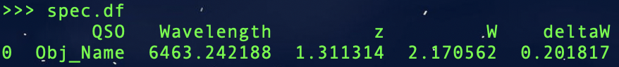
A DataFrame is saved as the df attribute, and if the specified spectral is detected in the spectrum, then the data will be appended to the DataFrame. Note that by default the save_all class attribute is set to True, which will save entries for which there are no positive detections; these entries will contain the qso_name followed by ‘None’ values. If save_all is set to False, only spectra with positive detection will be appended to the df attribute.
After running the process_spectrum method, the instantiated class will contain the continuum and continuum_err array attributes. These will be used automatically when calling the plot method:
spec.plot(include='both', highlight=True, xlim=(6432,6519), ylim=(-0.2,8), savefig=False)
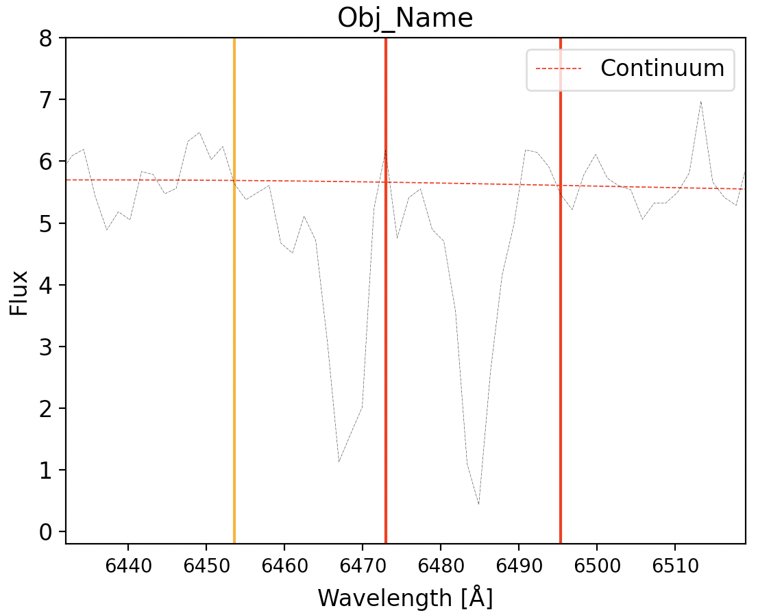
The include parameter can be set to either ‘spectrum’ to plot the flux only, ‘continuum’ to display only the continuum fit, or ‘both’ for both options.
IMPORTANT: If no line is found it is possible that the continuum was insufficiently estimated as a result of low S/N, therefore it is avised to experiment with different program parameters to identify those appropriate for your data. In this example, the redshift of the absorber and hence the equivalent widths are slightly off, to facilitate the tuning procedure the program contains an optimization routine. If the redshift of the absorber is known, you can enter this into the optimize class method which will optimize the class parameters until this redshift is successfully retrieved:
z_element = 1.31252 # As per Cooksey+13

# Parameters to tune
halfWindow = (10, 100)
region_size = (10, 200)
resolution_element = 3
savgol_window_size = (10, 200)
savgol_poly_order = (1, 7)
N_sig_limits = (0.1, 5)
N_sig_line1 = (0.1, 5)
N_sig_line2 = (0.1, 5)

n_trials = 250 # Will perform 250 iterations/parameter trials
threshold = 0.005 # Will stop the optimization if the calculated redshift is within this tolerance

# Start the optimization
spec.optimize(lam, flux, flux_err, z_qso=z_qso, z_element=z_element, halfWindow=halfWindow, region_size=region_size,
    resolution_element=resolution_element, savgol_window_size=savgol_window_size, savgol_poly_order=savgol_poly_order,
    N_sig_limits=N_sig_limits, N_sig_line1=N_sig_line1, N_sig_line2=N_sig_line2, n_trials=n_trials, threshold=threshold, show_progress_bar=True)
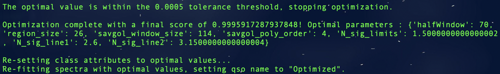
In the above example. the parameters designated as tuples will be tuned according to this specified range. Parameters entered as single values (like the resolution element) will not be tuned and the input value will be applied instead. The n_trials parameter will determine how many optimization iterations to perform, which will be driven according to the input z_element – the optimization will stop upon reaching this value or if the threshold tolerance is met.
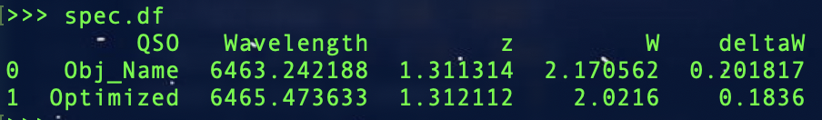
With the optimal values we can reproduce the results from Cooksey+13:
This spectra also contains a CIV absorber at a redshift of z_civ = 1.52755, with an equivalent witdh of 0.567. Below we demonstrate how to configure the program for this line’s detection, note the rest_wavelenght_1 and rest_wavelenght_2 are now set accordingly for this doublet:
import numpy as np
from astropy.io import fits
from LineDetect import spectra_processor

spec = spectra_processor.Spectrum(resolution_range=(1500, 2538.46), rest_wavelength_1=1548.19, rest_wavelength_2=1550.77)

hdu = fits.open('spec-0650-52143-0199.fits')
lam, flux = 10**hdu[1].data['loglam'], hdu[1].data['flux']
ivar = hdu[1].data['ivar']
flux_err = np.sqrt(np.where(ivar > 0, 1 / ivar, np.inf))
z_qso = hdu[2].data['Z'][0]

z_element = 1.52755

halfWindow = (10, 100)
region_size = (10, 200)
resolution_element = 3
savgol_window_size = (10, 200)
savgol_poly_order = (1, 7)
N_sig_limits = (0.1, 5)
N_sig_line1 = (0.1, 5)
N_sig_line2 = (0.1, 5)

n_trials = 250
threshold=0.005

spec.optimize(lam, flux, flux_err, z_qso=z_qso, z_element=z_element, halfWindow=halfWindow, region_size=region_size, resolution_element=resolution_element,
    savgol_window_size=savgol_window_size, savgol_poly_order=savgol_poly_order, N_sig_limits=N_sig_limits, N_sig_line1=N_sig_line1, N_sig_line2=N_sig_line2,
    n_trials=n_trials, threshold=threshold, show_progress_bar=True)
2) Directory
As the DataFrame, df, appends new results every time (if save_file is set to True), files from a directory can be processed at any point, although ccurrently the system supports only the fits format with the following header information:
[0].header[‘Z’] is the redshift of the source, [0].data is the 1-D flux, and hdu[1].data the corresponding flux error.
[0].header must also contain the redshift information (float) and the appropriate coordinate conversion factor so as to invoke the Astropy World Coordinate System
To load fits files from a directory, set the directory attribute and call the process_files method – note that the qso_name that will be saved to the DataFrame will be automatically set to the file name.
spec.directory = '/Path/to/dir/'
spec.process_files()

#Process another directory, the identified lines will be appended to the DataFrame
spec.directory = '/Path/to/different/dir/'
spec.process_files()
Unlike when processing single spectra with process_spectrum, this method does not save continuum and continuum_err attributes, therefore the plot method cannot be called to view these samples, they will have to loaded individually for plotting purposes.